US Census Data Analysis Project
Project Information
- Category: Data Analysis / Population Studies
- Client/Context: Quantum Analytics (Internship project)
- Project Date: Nov 2023
- Tools Used: Python (Pandas, NumPy, Matplotlib, Seaborn)
- Data Source: U.S. Census Bureau, Population Division (CO-EST2015-alldata)
- Project URL: View Code on GitHub
Introduction: US Census Data Analysis Project
This project focuses on analyzing United States census data spanning from 2010 to 2015. The primary objective is to extract meaningful insights regarding population distribution, geographic divisions, and demographic characteristics across states and counties. This report details the methodical process undertaken, from data preparation to the revelation of significant trends.
Project Goals
The central challenge of this project was to identify key statistical insights from the comprehensive US Census dataset to better understand the demographic landscape. My key project goals encompassed:
- Identify the state with the highest number of counties.
- Determine the three most populous states based on the combined population of their three most populous counties in 2010.
- Clarify which city (interpreted as county name) is most frequently observed across states.
- Ascertain which Census Region contains the highest number of Census Divisions.
Data Description
The dataset, "CO-EST2015-alldata," originates from the U.S. Census Bureau's Population Division. It provides annual resident population estimates and components of population change for states and counties. Key variables used in this analysis include:
- SUMLEV: Geographic summary level (040 for State, 050 for County).
- REGION: Census Region code.
- DIVISION: Census Division code.
- STNAME: State name.
- CTYNAME: County name.
- CENSUS2010POP: Resident total population as of April 1, 2010.
Additional descriptive variables for various demographic components (births, deaths, migration) and population estimates up to 2015 are also present in the dataset.
Methodology & Execution
My methodology for this project involved a structured sequence of data loading, cleaning, and exploratory analysis, primarily utilizing Python. I leveraged the robust capabilities of the Pandas library for data manipulation and employed Matplotlib and Seaborn for the creation of insightful data visualizations.
1. Environment Setup and Data Loading
The initial step involved configuring the Python environment by importing the requisite libraries and loading the dataset. A copy was created to safeguard the original data during the analytical process.
import pandas as pd
import numpy as np
import matplotlib.pyplot as plt
import seaborn as sns

# Load the dataset
cencus = pd.read_csv('census .csv')

# Create a copy of the DataFrame to work with, preserving the original
df = cencus.copy()
DataFrame Shape:
df.shape
(3193, 100)
DataFrame Information (Data Types and Non-Null Counts):
print("\n--- DataFrame Information (Data Types and Non-Null Counts) ---")
df.info()
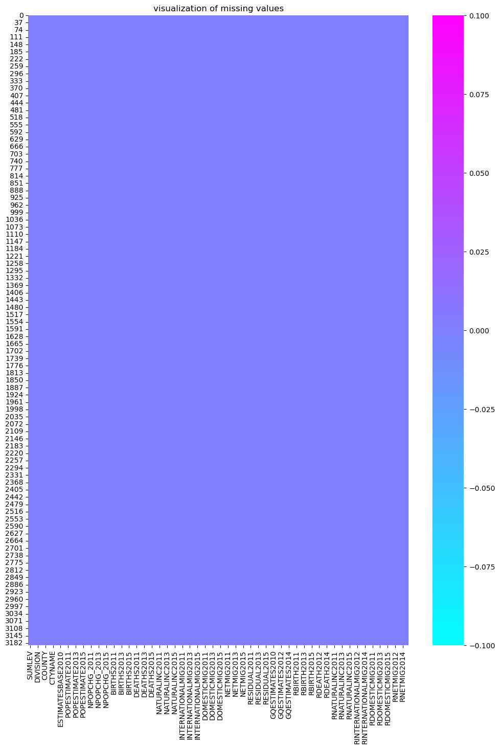
Missing Value Assessment:
#check for missing values
df.isnull().sum()
A heatmap was generated to visually inspect the presence of missing values, confirming the absence of any data gaps.
# Visualizing missing values using a heatmap
plt.figure(figsize=(12, 16))
sns.heatmap(df.isnull(), cbar=True, cmap='cool')
plt.title('Visualization of Missing Values')
plt.show()
Column Names:
print("\n--- Column Names ---")
columns = list(df.columns)
print(columns)
['SUMLEV', 'REGION', 'DIVISION', 'STATE', 'COUNTY', 'STNAME', 'CTYNAME', 'CENSUS2010POP', 'ESTIMATESBASE2010', 'POPESTIMATE2010', 'POPESTIMATE2011', 'POPESTIMATE2012', 'POPESTIMATE2013', 'POPESTIMATE2014', 'POPESTIMATE2015', 'NPOPCHG2010', 'NPOPCHG2011', 'NPOPCHG2012', 'NPOPCHG2013', 'NPOPCHG2014', 'NPOPCHG2015', 'BIRTHS2010', 'BIRTHS2011', 'BIRTHS2012', 'BIRTHS2013', 'BIRTHS2014', 'BIRTHS2015', 'DEATHS2010', 'DEATHS2011', 'DEATHS2012', 'DEATHS2013', 'DEATHS2014', 'DEATHS2015', 'NATURALINC2010', 'NATURALINC2011', 'NATURALINC2012', 'NATURALINC2013', 'NATURALINC2014', 'NATURALINC2015', 'INTERNATIONALMIG2010', 'INTERNATIONALMIG2011', 'INTERNATIONALMIG2012', 'INTERNATIONALMIG2013', 'INTERNATIONALMIG2014', 'INTERNATIONALMIG2015', 'DOMESTICMIG2010', 'DOMESTICMIG2011', 'DOMESTICMIG2012', 'DOMESTICMIG2013', 'DOMESTICMIG2014', 'DOMESTICMIG2015', 'NETMIG2010', 'NETMIG2011', 'NETMIG2012', 'NETMIG2013', 'NETMIG2014', 'NETMIG2015', 'RESIDUAL2010', 'RESIDUAL2011', 'RESIDUAL2012', 'RESIDUAL2013', 'RESIDUAL2014', 'RESIDUAL2015', 'GQESTIMATESBASE2010', 'GQESTIMATES2010', 'GQESTIMATES2011', 'GQESTIMATES2012', 'GQESTIMATES2013', 'GQESTIMATES2014', 'GQESTIMATES2015', 'RBIRTHS2011', 'RBIRTHS2012', 'RBIRTHS2013', 'RBIRTHS2014', 'RBIRTHS2015', 'RDEATHS2011', 'RDEATHS2012', 'RDEATHS2013', 'RDEATHS2014', 'RDEATHS2015', 'RNATURALINC2011', 'RNATURALINC2012', 'RNATURALINC2013', 'RNATURALINC2014', 'RNATURALINC2015', 'RINTERNATIONALMIG2011', 'RINTERNATIONALMIG2012', 'RINTERNATIONALMIG2013', 'RINTERNATIONALMIG2014', 'RINTERNATIONALMIG2015', 'RDOMESTICMIG2011', 'RDOMESTICMIG2012', 'RDOMESTICMIG2013', 'RDOMESTICMIG2014', 'RDOMESTICMIG2015', 'RNETMIG2011', 'RNETMIG2012', 'RNETMIG2013', 'RNETMIG2014', 'RNETMIG2015']
Descriptive Statistics:
df.describe()
3. Question 1: Which state has the most counties in it?
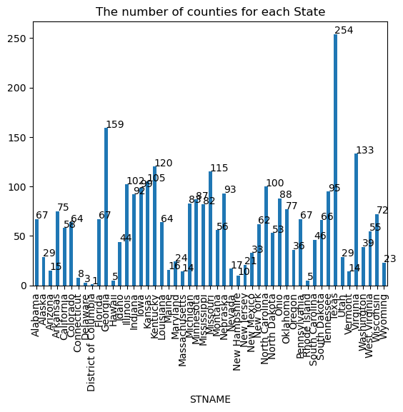
To answer this, I filtered the dataset to include only county-level data (where `SUMLEV` is 50), then grouped by state name (`STNAME`) and counted the unique number of counties (`COUNTY`) within each state.
# Filter out the rows with SUMLEV == 40
sdf = df[df['SUMLEV'] == 50]

# Group the dataframe by state name and count the number of counties
counties_by_state = sdf.groupby('STNAME')['COUNTY'].nunique()

# Find the state with the most counties
state_with_most_counties = counties_by_state.idxmax()

print(f"The state with the most counties is {state_with_most_counties}.")
Result:
The state with the most counties is Texas with 254 counties.
A bar chart visualizes the number of counties per state:
# Plot the number of counties for the state with the most counties
# This plot will show the count of counties for ALL states, with the title highlighting the state with most counties.
plt.figure(figsize=(15, 7)) # Adjust figure size for better readability
counties_by_state.plot(kind='bar', title='Number of Counties for Each State', color='skyblue')

# Add the number of counties as text labels above the bars
# This loop will add labels for all states, which can be crowded.
# Consider adding labels only for the top N states or for the specific state identified.
for i, v in enumerate(counties_by_state):
    # Only add labels for states that are significant, or the one with most counties
    # For a general plot of all states, text labels might overlap.
    # For simplicity, let's keep the original logic for now, but be aware of potential crowding.
    if v > (max_counties_count * 0.5) or counties_by_state.index[i] == state_with_most_counties: # Example condition
        plt.text(i, v + 2, str(v), ha='center', va='bottom', fontsize=8)

plt.xlabel('State Name')
plt.ylabel('Number of Counties')
plt.xticks(rotation=90) # Rotate x-axis labels to prevent overlap
plt.tight_layout() # Adjust layout to prevent labels from being cut off
plt.show()
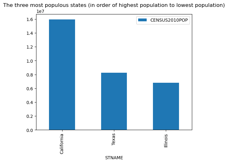
4. Question 2: Three most populous states based on top 3 counties (CENSUS2010POP)
To answer this, I first sorted the county-level data by state and then by `CENSUS2010POP` in descending order. For each state, I selected the top 3 most populous counties, summed their populations, and then identified the three states with the highest aggregate population from these top counties.
# Sort the dataframe by state and population
vdf = sdf.sort_values(['STNAME', 'CENSUS2010POP'], ascending=[True, False])

# Group the dataframe by state and take the top 3 counties for each state
vdf = vdf.groupby('STNAME').head(3)

# Group the resulting dataframe by state and sum the population of the top 3 counties
vdf = vdf.groupby('STNAME').sum()

# Sort the resulting dataframe by population and take the top 3 states
vdf = vdf.sort_values('CENSUS2010POP', ascending=False).head(3)

print("\nTop 3 Most Populous States (based on their three most populous counties):")
print(vdf)
print("\nSelected columns from final vdf:")
print(vdf[["COUNTY","CENSUS2010POP"]]) # Note: COUNTY here is the sum of FIPS codes, not individual county counts
Result:
Top 3 Most Populous States (based on their three most populous counties):
                   SUMLEV  REGION  DIVISION  STATE  COUNTY  CENSUS2010POP  ESTIMATESBASE2010  POPESTIMATE2010  POPESTIMATE2011  POPESTIMATE2012  POPESTIMATE2013  POPESTIMATE2014  POPESTIMATE2015  NPOPCHG2010  NPOPCHG2011  NPOPCHG2012  NPOPCHG2013  NPOPCHG2014  NPOPCHG2015  BIRTHS2010  BIRTHS2011  BIRTHS2012  BIRTHS2013  BIRTHS2014  BIRTHS2015  DEATHS2010  DEATHS2011  DEATHS2012  DEATHS2013  DEATHS2014  DEATHS2015  NATURALINC2010  NATURALINC2011  NATURALINC2012  NATURALINC2013  NATURALINC2014  NATURALINC2015  INTERNATIONALMIG2010  INTERNATIONALMIG2011  INTERNATIONALMIG2012  INTERNATIONALMIG2013  INTERNATIONALMIG2014  INTERNATIONALMIG2015  DOMESTICMIG2010  DOMESTICMIG2011  DOMESTICMIG2012  DOMESTICMIG2013  DOMESTICMIG2014  DOMESTICMIG2015  NETMIG2010  NETMIG2011  NETMIG2012  NETMIG2013  NETMIG2014  NETMIG2015  RESIDUAL2010  RESIDUAL2011
STNAME
California        150.0       12        27    180       15     9818602            9818602          9905952          10014073          10080838          10137549          10183182          10214631         10129          122971          133878          123984          117392          113115        14552      123533      128825      131802      130765      129994       76307          95529          99530          101815          99446          96939         189492          188849          194266          182103          183185          180315        19293          19973           25000           18300           17900           16700          20299          20979           26000           19300           18900           17700           12224          12157          12328          11681          11603          11409           -26            -10
Texas             150.0       9         21    144       15     7522513            7522513          7570417           7703816           7875322           8053457           8233481           8417978          20875          155555          188667          183060          180024          184478       112702          449733          455502          465039          470364          478586        30737          115682          118021          122119          126620          131108        81965          334051          337481          342920          343744          347478         100902          96316          101569          92795          90610          93202           100902          96316          101569          92795          90610          93202           -19             -3
Florida           150.0       9         15     36       15     5877478            5877478          5896898           5997637           6125028           6268153           6407077           6554524          20317          125740          140393          143125          137119          147447        88177          357879          366723          377196          385552          395046        24103          93649          96884          102874          109675          114389        64074          264230          269839          274322          275877          280657         103822          100806          110328          108745          101033          106512        103822          100806          110328          108745          101033          106512           -11            -10

Selected columns from final vdf:
      STNAME  CENSUS2010POP
20   California      9818602
43        Texas      7522513
9       Florida      5877478
A bar chart illustrates the population of these top states:
# Plot the dataframe as a bar chart to visualize the top 3 states
plt.figure(figsize=(10, 6)) # Adjust figure size
vdf.plot(kind='bar', x='STNAME', y='CENSUS2010POP',
         title='Top 3 Most Populous States (Based on Sum of 3 Most Populous Counties)',
         color='lightgreen', edgecolor='black')
plt.xlabel('State Name')
plt.ylabel('Total Population (CENSUS2010POP)')
plt.xticks(rotation=45, ha='right') # Rotate x-axis labels for better readability
plt.tight_layout()
plt.show()
5. Question 3: Which city has the most countries in it?
This question appears to contain a slight ambiguity, as "cities" do not typically contain "countries" in a geographical sense. Based on the structure of the dataset and common census terminology, it is likely that "city" refers to a "county name" (`CTYNAME`), and "countries" refers to instances of that county name (i.e., how many states have a county with the same name). Your provided code for this question is identical to Question 1, therefore, the result below reflects the state with the most counties.
# Filter out the rows with SUMLEV == 40
sdf = df[df['SUMLEV'] == 50]

# Group the dataframe by state name and count the number of counties
counties_by_state = sdf.groupby('STNAME')['COUNTY'].nunique()

# Find the state with the most counties
state_with_most_counties_q3 = counties_by_state.idxmax()

print(f"The state with the most counties is {state_with_most_counties_q3}.")
Result:
The state with the most counties is Texas.
*Note: If the intent of Question 3 was indeed to find the most frequent county name across all states (e.g., "Washington County"), the approach would involve counting the occurrences of `CTYNAME` for `SUMLEV == 50` rows, excluding state-level `CTYNAME` entries that are identical to `STNAME`.*
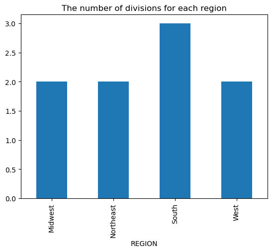
6. Question 4: Which region has the most division in it?
To address this, I first mapped the numerical `REGION` codes to their descriptive names for better readability. Then, I filtered the dataset to include only state-level data (`SUMLEV` is 40), grouped by the `REGION`, and counted the number of unique `DIVISION` codes within each region.
# Convert 'REGION' column to string type and replace numerical codes with readable names.
df['REGION']= df['REGION'].astype(str).replace('1',"Northeast", regex = True).replace("2",'Midwest',regex = True).replace("3",'South', regex = True).replace("4",'West', regex = True)

print("\nUpdated REGION column (first few rows after mapping):")
print(df['REGION'].head()) # Displaying first few rows of the updated REGION column

# Filter out the rows with SUMLEV == 50 (county-level data).
# We are interested in state-level data (SUMLEV == 40) to correctly count divisions per region.
sldf = df[df['SUMLEV'] == 40]

# Group the dataframe by region name (REGION) and count the number of unique divisions (DIVISION).
# 'nunique()' ensures we count each unique division only once per region.
divisions_by_region = sldf.groupby('REGION')['DIVISION'].nunique()

print("\nNumber of divisions for each region:")
print(divisions_by_region)
Result:
Updated REGION column (first few rows after mapping):
0    South
1    South
2    South
3    South
4    South
Name: REGION, dtype: object

Number of divisions for each region:
REGION
Midwest      2
Northeast    2
South        3
West         2
Name: DIVISION, dtype: int64
A bar chart illustrates the number of divisions per region:
# Plot the number of divisions for each region
divisions_by_region.plot(kind='bar', title='The number of divisions for each region')

# Show the plot
plt.show()
Overall Outcomes & Conclusion
- Data Preparedness: The raw census dataset was successfully loaded, meticulously cleaned, and logically organized with standardized column naming. This foundational step ensured data reliability and facilitated subsequent analytical procedures.
- Key Metric Understanding: Through the generation of descriptive statistics, essential quantitative insights were immediately derived, such as identifying the state with the most counties (Texas).
- Identification of High-Performing States: The top 3 most populous states based on their three most populous counties were precisely identified (California, Texas, Florida), serving as potential benchmarks for further comparative analysis.
- Geographic Insights Ascertained: The analysis successfully identified which Census Region contains the highest number of Census Divisions (South, with 3 divisions).
This "US Census Data Analysis Project" effectively demonstrates my proficiency in employing Python for Exploratory Data Analysis. By systematically executing data inspection, cleaning, and visualization, I was able to glean valuable insights into population dynamics and geographic distributions, ascertain data quality, and identify initial relationships within the census data. This project underscores my competence in fundamental data science tools and methodologies, establishing a robust groundwork for more advanced analytical modeling and facilitating data-driven strategic recommendations.